pandas - DataFrame Intro
pandas - DataFrame Intro
A very useful Python package is pandas, which is an open source library providing high-performance, easy-to-use data structures and data analysis tools for Python. pandas stands for panel data, a term borrowed from econometrics and is an efficient library for data analysis with an emphasis on tabular data. pandas has two major classes, the DataFrame class with two-dimensional data objects and tabular data organized in columns and the class Series with a focus on one-dimensional data objects. Both classes allow you to index data easily as we will see in the examples below. pandas allows you also to perform mathematical operations on the data, spanning from simple reshapings of vectors and matrices to statistical operations.
The following simple example shows how we can, in an easy way make tables of our data. Here we define a data set which includes names, place of birth and date of birth, and displays the data in an easy to read way. We will see repeated use of pandas, in particular in connection with classification of data.
import pandas as pd
from IPython.display import display
data = {'First Name': ["Frodo", "Bilbo", "Aragorn II", "Samwise"],
        'Last Name': ["Baggins", "Baggins","Elessar","Gamgee"],
        'Place of birth': ["Shire", "Shire", "Eriador", "Shire"],
        'Date of Birth T.A.': [2968, 2890, 2931, 2980]
        }
data_pandas = pd.DataFrame(data)
display(data_pandas)
| First Name | Last Name | Place of birth | Date of Birth T.A. | |
|---|---|---|---|---|
| 0 | Frodo | Baggins | Shire | 2968 |
| 1 | Bilbo | Baggins | Shire | 2890 |
| 2 | Aragorn II | Elessar | Eriador | 2931 |
| 3 | Samwise | Gamgee | Shire | 2980 |
In the above we have imported pandas with the shorthand pd, the latter has become the standard way we import pandas. We make then a list of various variables and reorganize the aboves lists into a DataFrame and then print out a neat table with specific column labels as Name, place of birth and date of birth. Displaying these results, we see that the indices are given by the default numbers from zero to three. pandas is extremely flexible and we can easily change the above indices by defining a new type of indexing as
data_pandas = pd.DataFrame(data,index=['Frodo','Bilbo','Aragorn','Sam'])
display(data_pandas)
| First Name | Last Name | Place of birth | Date of Birth T.A. | |
|---|---|---|---|---|
| Frodo | Frodo | Baggins | Shire | 2968 |
| Bilbo | Bilbo | Baggins | Shire | 2890 |
| Aragorn | Aragorn II | Elessar | Eriador | 2931 |
| Sam | Samwise | Gamgee | Shire | 2980 |
Thereafter we display the content of the row which begins with the index Aragorn
display(data_pandas.loc['Aragorn'])
First Name            Aragorn II
Last Name                Elessar
Place of birth           Eriador
Date of Birth T.A.          2931
Name: Aragorn, dtype: object
We can easily append data to this, for example
new_hobbit = {'First Name': ["Peregrin"],
              'Last Name': ["Took"],
              'Place of birth': ["Shire"],
              'Date of Birth T.A.': [2990]
              }
data_pandas=data_pandas.append(pd.DataFrame(new_hobbit, index=['Pippin']))
display(data_pandas)
| First Name | Last Name | Place of birth | Date of Birth T.A. | |
|---|---|---|---|---|
| Frodo | Frodo | Baggins | Shire | 2968 |
| Bilbo | Bilbo | Baggins | Shire | 2890 |
| Aragorn | Aragorn II | Elessar | Eriador | 2931 |
| Sam | Samwise | Gamgee | Shire | 2980 |
| Pippin | Peregrin | Took | Shire | 2990 |
Here are other examples where we use the DataFrame functionality to handle arrays, now with more interesting features for us, namely numbers. We set up a matrix of dimensionality \(10\times 5\) and compute the mean value and standard deviation of each column. Similarly, we can perform mathematial operations like squaring the matrix elements and many other operations.
import numpy as np
import pandas as pd
from IPython.display import display
np.random.seed(100)
# setting up a 10 x 5 matrix
rows = 10
cols = 5
a = np.random.randn(rows,cols)
df = pd.DataFrame(a)
display(df)
print(df.mean())
print(df.std())
display(df**2)
| 0 | 1 | 2 | 3 | 4 | |
|---|---|---|---|---|---|
| 0 | -1.749765 | 0.342680 | 1.153036 | -0.252436 | 0.981321 |
| 1 | 0.514219 | 0.221180 | -1.070043 | -0.189496 | 0.255001 |
| 2 | -0.458027 | 0.435163 | -0.583595 | 0.816847 | 0.672721 |
| 3 | -0.104411 | -0.531280 | 1.029733 | -0.438136 | -1.118318 |
| 4 | 1.618982 | 1.541605 | -0.251879 | -0.842436 | 0.184519 |
| 5 | 0.937082 | 0.731000 | 1.361556 | -0.326238 | 0.055676 |
| 6 | 0.222400 | -1.443217 | -0.756352 | 0.816454 | 0.750445 |
| 7 | -0.455947 | 1.189622 | -1.690617 | -1.356399 | -1.232435 |
| 8 | -0.544439 | -0.668172 | 0.007315 | -0.612939 | 1.299748 |
| 9 | -1.733096 | -0.983310 | 0.357508 | -1.613579 | 1.470714 |
0   -0.175300
1    0.083527
2   -0.044334
3   -0.399836
4    0.331939
dtype: float64
0    1.069584
1    0.965548
2    1.018232
3    0.793167
4    0.918992
dtype: float64
| 0 | 1 | 2 | 3 | 4 | |
|---|---|---|---|---|---|
| 0 | 3.061679 | 0.117430 | 1.329492 | 0.063724 | 0.962990 |
| 1 | 0.264421 | 0.048920 | 1.144993 | 0.035909 | 0.065026 |
| 2 | 0.209789 | 0.189367 | 0.340583 | 0.667239 | 0.452553 |
| 3 | 0.010902 | 0.282259 | 1.060349 | 0.191963 | 1.250636 |
| 4 | 2.621102 | 2.376547 | 0.063443 | 0.709698 | 0.034047 |
| 5 | 0.878123 | 0.534362 | 1.853835 | 0.106431 | 0.003100 |
| 6 | 0.049462 | 2.082875 | 0.572069 | 0.666597 | 0.563167 |
| 7 | 0.207888 | 1.415201 | 2.858185 | 1.839818 | 1.518895 |
| 8 | 0.296414 | 0.446453 | 0.000054 | 0.375694 | 1.689345 |
| 9 | 3.003620 | 0.966899 | 0.127812 | 2.603636 | 2.162999 |
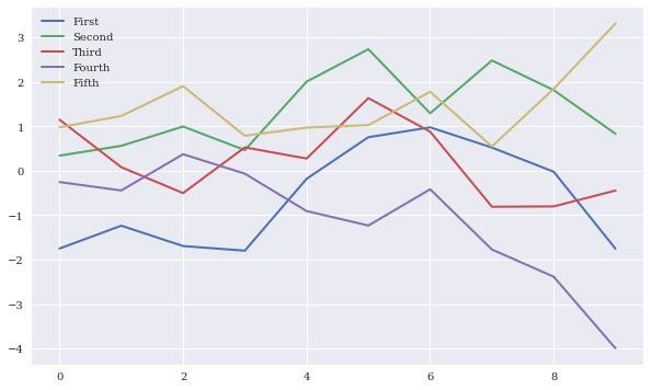
Thereafter we can select specific columns only and plot final results
df.columns = ['First', 'Second', 'Third', 'Fourth', 'Fifth']
df.index = np.arange(10)
display(df)
print(df['Second'].mean() )
print(df.info())
print(df.describe())
from pylab import plt, mpl
plt.style.use('seaborn')
mpl.rcParams['font.family'] = 'serif'
df.cumsum().plot(lw=2.0, figsize=(10,6))
plt.show()
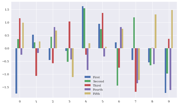
df.plot.bar(figsize=(10,6), rot=15)
plt.show()
| First | Second | Third | Fourth | Fifth | |
|---|---|---|---|---|---|
| 0 | -1.749765 | 0.342680 | 1.153036 | -0.252436 | 0.981321 |
| 1 | 0.514219 | 0.221180 | -1.070043 | -0.189496 | 0.255001 |
| 2 | -0.458027 | 0.435163 | -0.583595 | 0.816847 | 0.672721 |
| 3 | -0.104411 | -0.531280 | 1.029733 | -0.438136 | -1.118318 |
| 4 | 1.618982 | 1.541605 | -0.251879 | -0.842436 | 0.184519 |
| 5 | 0.937082 | 0.731000 | 1.361556 | -0.326238 | 0.055676 |
| 6 | 0.222400 | -1.443217 | -0.756352 | 0.816454 | 0.750445 |
| 7 | -0.455947 | 1.189622 | -1.690617 | -1.356399 | -1.232435 |
| 8 | -0.544439 | -0.668172 | 0.007315 | -0.612939 | 1.299748 |
| 9 | -1.733096 | -0.983310 | 0.357508 | -1.613579 | 1.470714 |
0.08352721390288316
<class 'pandas.core.frame.DataFrame'>
Int64Index: 10 entries, 0 to 9
Data columns (total 5 columns):
 #   Column  Non-Null Count  Dtype
---  ------  --------------  -----
 0   First   10 non-null     float64
 1   Second  10 non-null     float64
 2   Third   10 non-null     float64
 3   Fourth  10 non-null     float64
 4   Fifth   10 non-null     float64
dtypes: float64(5)
memory usage: 480.0 bytes
None
           First     Second      Third     Fourth      Fifth
count  10.000000  10.000000  10.000000  10.000000  10.000000
mean   -0.175300   0.083527  -0.044334  -0.399836   0.331939
std     1.069584   0.965548   1.018232   0.793167   0.918992
min    -1.749765  -1.443217  -1.690617  -1.613579  -1.232435
25%    -0.522836  -0.633949  -0.713163  -0.785061   0.087887
50%    -0.280179   0.281930  -0.122282  -0.382187   0.463861
75%     0.441264   0.657041   0.861676  -0.205231   0.923602
max     1.618982   1.541605   1.361556   0.816847   1.470714
We can produce a \(4\times 4\) matrix
b = np.arange(16).reshape((4,4))
print(b)
df1 = pd.DataFrame(b)
print(df1)
[[ 0  1  2  3]
 [ 4  5  6  7]
 [ 8  9 10 11]
 [12 13 14 15]]
    0   1   2   3
0   0   1   2   3
1   4   5   6   7
2   8   9  10  11
3  12  13  14  15
and many other operations.
The Series class is another important class included in pandas. You can view it as a specialization of DataFrame but where we have just a single column of data. It shares many of the same features as _DataFrame. As with DataFrame, most operations are vectorized, achieving thereby a high performance when dealing with computations of arrays, in particular labeled arrays. As we will see below it leads also to a very concice code close to the mathematical operations we may be interested in. For multidimensional arrays, we recommend strongly xarray. xarray has much of the same flexibility as pandas, but allows for the extension to higher dimensions than two. We will see examples later of the usage of both pandas and xarray.
In order to study various Machine Learning algorithms, we need to access data. Acccessing data is an essential step in all machine learning algorithms. In particular, setting up the so-called design matrix (to be defined below) is often the first element we need in order to perform our calculations. To set up the design matrix means reading (and later, when the calculations are done, writing) data in various formats, The formats span from reading files from disk, loading data from databases and interacting with online sources like web application programming interfaces (APIs).
In handling various input formats, as discussed above, we will mainly stay with pandas, a Python package which allows us, in a seamless and painless way, to deal with a multitude of formats, from standard csv (comma separated values) files, via excel, html to hdf5 formats. With pandas and the DataFrame and Series functionalities we are able to convert text data into the calculational formats we need for a specific algorithm. And our code is going to be pretty close the basic mathematical expressions.